Backtesting 12-month SMA investing strategy with Pandas
Published by Danny van Kooten on .
In my quest to learn more about investing, I came across this post. The author writes “How One Simple Rule Can Beat Buy and Hold Investing” and then explains how following the trend is likely to beat a more traditional buy and hold investment approach.
Intrigued, I decided to dive into the data to see if I could replicate his results.
In this post I’ll walk you through the code and results for backtesting a 12-month simple moving average trend strategy on S&P 500 stock market data.
We’ll compare entering the market when it is trending up and moving to cash when it is trending down to simply staying invested at all times. The latter approach is known as buy & hold, or HODL depending on what corner of the internet you’re from.
Obtaining data on daily closing prices for the S&P 500
First things first, we need data.
Yahoo Finance provides us with historical data for the S&P 500 as far back as 1960. Let’s start out with parsing the CSV download into a DataFrame so we can get to work.
%matplotlib inline
import pandas as pd

sp500 = pd.read_csv('data/SP500.csv', sep=',', parse_dates=True, index_col='Date', usecols=['Adj Close', 'Date'])
sp500.head()| Date | Adj Close |
|---|---|
| 1960-01-04 | 59.910000 |
| 1960-01-05 | 60.389999 |
| 1960-01-06 | 60.130001 |
| 1960-01-07 | 59.689999 |
| 1960-01-08 | 59.500000 |
Calculating the 12 month simple moving average
To test our trend strategy later on, we need the daily change (in %) and the 12-month simple moving average.
sp500['Pct Change'] = sp500['Adj Close'].pct_change()
sp500['SMA 365'] = sp500['Adj Close'].rolling(window=365).mean()
sp500.dropna().head()| Date | Adj Close | Pct Change | SMA 365 |
|---|---|---|---|
| 1961-06-14 | 65.980003 | 0.002736 | 58.350521 |
| 1961-06-15 | 65.690002 | -0.004395 | 58.366356 |
| 1961-06-16 | 65.180000 | -0.007764 | 58.379479 |
| 1961-06-19 | 64.580002 | -0.009205 | 58.391671 |
| 1961-06-20 | 65.150002 | 0.008826 | 58.406630 |
This leaves us with all the data we need to compare our two investment strategies.
Defining the trend strategy
To recap, we want to invest when the trend is moving up, ie when the stock price is higher than the average price over the last 12 months. When the stock is traded at a price lower than the moving average, we move to cash.
Let’s add a column to our dataframe indicating whether the criteria for our trend strategy is met.
sp500['Criteria'] = sp500['Adj Close'] >= sp500['SMA 365']
sp500['Criteria'].value_counts()
True 10577
False 4032
Name: Criteria, dtype: int64This tells us that on our entire dataset, our criteria was met on 10577 of the market’s trading days.
Calculating our investment return
To calculate the return for our benchmark buy & hold strategy, all we need to do is calculate the cumulative product of the daily change in prices.
Let’s assume an initial investment of $100 and calculate the return if we were to hold for the entire time period.
sp500['Buy & Hold'] = 100 * (1 + sp500['Pct Change']).cumprod()To calculate the return for our strategy, we should only add the compounded return for the days on which we are actually in the market.
On all other days the cash value of our investment remains unchanged.
sp500['Trend'] = 100 * (1 + ( sp500['Criteria'].shift(1) * sp500['Pct Change'] )).cumprod()Let’s plot the values of both strategies in a single graph so that we can compare performances.
ax = sp500[['Trend', 'Buy & Hold']].plot(grid=True, kind='line', title="Trend (12 month SMA) vs. Buy & Hold", logy=True)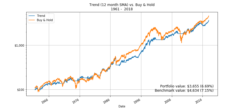
This shows us that a simple buy & hold investing approach actually outperformed our trend strategy when looking at the S&P 500 market data for 1960 to early 2018.
Seeking outperformance
Looking at the graph above, you can see that the trend did well during ongoing bear markets but sometimes failed to pick up on quick market recoveries.
So let’s cheat a little and look at just “the lost decade”, which contains not just one but two relatively long bear markets!
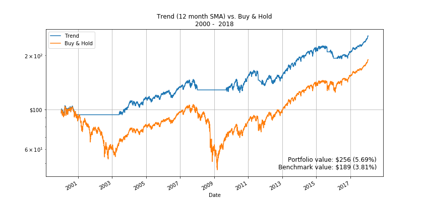
This shows us that our trend strategy resulted in considerable outperformance during these 2 decades, but only because of the two bear markets.
Conclusion: Trend following over Buy & Hold?
After playing with the data and looking at performance of the 2 strategies over different time periods, I think it’s safe to say that simple buy and hold is the way to go for most individual investors. Especially as the above does not take transaction costs into account just yet.
With some hindsight we can make the trend following model outperform, but in real life we obviously do not have that luxury. Luckily, buy and hold has always made up for the difference in returns, even if you bought in just before 2 decades of bear markets.
You can find the complete Jupyter Notebook for this post here.